SIGSAM Challenges
In February 1997, Fee and Monogan proposed ten numerical problems that seem to be solvable with typical numerical libraries. They write:
“[We present] some problems that appear at first glance to be purely numerical, that is they look like they should be solvable by using a purely numerical package. However, you may find that this just leads to an error message when you try to solve them using a purely numerical package. Can our computer algebra systems come to the rescue and solve the following problems?”
Almost 30 years later, we present solutions to these problems with modern programs.
Problem 1
What is a 4 significant digit approximation to the condition number of the 256x256 Hilbert matrix?
- the \(n \times n\) Hilbert matrix is the matrix \(H = (h_{ij})_{\substack {1 \le i \le n \\ 1 \le j \le n}}\) where \(h_{ij} = 1/(i+j-1)\)
- the condition number of a \(n \times n\) matrix \(A\) is defined to be \(\|A\|_2 \cdot \|A^{-1}\|_2\) with \(\| \cdot \|_2\) is the spectral norm
We first attempt to solve this problem with standard libraries:
import numpy as np

N = 256
H = np.array([[1./(i+j-1) for i in range(1, N+1)] for j in range(1, N+1)])
np.linalg.cond(H, p=2)
With this code, we get that the condition number \(c \; \dot= \; 1.9488855527466815 \cdot 10^{20}\) - however, we do not know how many digits are correct.
Some theory
We have for a real \(n \times n\) matrix \(A\), we have that \[ \| A \|_2 = \sup_{|x|_2 \ne 0} \frac{|Ax|_2}{|x|_2} = (\lambda_{\text{max}}(A^T A))^{1/2}\]
(Here, for a vector \(v = (v_1 \cdots v_n) \in \mathbb{R}^n\), \(|v|_2 = (\sum_{i=1}^n v_i^2)^{1/2}\) is the standard Euclidean norm and \(\lambda_{\text{max}}(M)\) represents the largest eigenvalue of \(M\))
Our plan of attack is as follows: - we can calculate \(\lambda_{\text{max}}\) via power iteration; this is useful as it is less expensive than other methods like calculating the characteristic polynomial - we have an explicit closed form of \((H^{-1})_{ij} = (-1)^{i+j} (i+j-1) \binom{n+i-1}{n-j} \binom{n+j-1}{n-i} \binom{i+j-2}{i-1}^2\) - we calculate \(c = \|H \|_2 \cdot \| H^{-1}\|_2\) with various working precisions and take agreeing digits as confirmation of precision
We first generate \(H\) and \(H^{-1}\):
import sympy
from math import comb as C

N = 256
H = sympy.Matrix([[sympy.Rational(1, i+j-1) for i in range(1, N+1)] for j in range(1, N+1)])
H_inv = sympy.Matrix( [[pow(-1, i+j)*(i+j-1)*C(N+i-1,N-j)*C(N+j-1, N-i)*C(i+j-2,i-1)**2 for i in range(1, N+1)] for j in range(1, N+1)] )
I = H_inv @ H; assert I == sympy.eye(N)
Immediately, we can see that the condition number given by
numpy is not accurate - note that the condition number of a
matrix and it’s inverse should be the same; however, we have:
In [58]: np.linalg.cond( np.array(H, dtype=float) )
Out[58]: np.float64(1.9488855527466815e+20)

In [59]: np.linalg.cond( np.array(H_inv, dtype=float) )
 ** On entry to DLASCL parameter number  4 had an illegal value
 ** On entry to DLASCL parameter number  5 had an illegal value
Out[59]: np.float64(inf)

In [60]: np.linalg.cond( np.linalg.inv( np.array(H, dtype=float) ) )
Out[60]: np.float64(7.398387590891174e+18)
Similarly, mpmath.cond fails to calculate the condition
number of this matrix:
In [65]: mpmath.cond( mpmath.matrix(H) )
---------------------------------------------------------------------------

/usr/local/lib/python3.12/dist-packages/mpmath/matrices/linalg.py in cond(ctx, A, norm)
    572         if norm is None:
    573             norm = lambda x: ctx.mnorm(x,1)
--> 574         return norm(A) * norm(ctx.inverse(A))
    575
    576     def lu_solve_mat(ctx, a, b):

/usr/local/lib/python3.12/dist-packages/mpmath/matrices/linalg.py in inverse(ctx, A, **kwargs)
    300             n = A.rows
    301             # get LU factorisation
--> 302             A, p = ctx.LU_decomp(A)
    303             cols = []
    304             # calculate unit vectors and solve corresponding system to get columns

/usr/local/lib/python3.12/dist-packages/mpmath/matrices/linalg.py in LU_decomp(ctx, A, overwrite, use_cache)
    140             ctx.swap_row(A, j, p[j])
    141             if ctx.absmin(A[j,j]) <= tol:
--> 142                 raise ZeroDivisionError('matrix is numerically singular')
    143             # calculate elimination factors and add rows
    144             for i in xrange(j + 1, n):

ZeroDivisionError: matrix is numerically singular
The following code calculates \(c\)
using mpmath for extended precision.
def calc_condition_number(prec: int):
    import mpmath
    mpmath.mp.dps = prec
    # Convert H, H^-1 to mpmath matrices with given precision
    H_mp = mpmath.matrix(H)
    H_inv_mp = mpmath.matrix(H_inv)

    # Calculate largest eigenvalue using power iteration
    import random
    random.seed(0)
    def power_iteration(M: mpmath.matrix, max_iter=1000):
        norm = lambda v: mpmath.sqrt(sum(map(lambda x: x**2, v)))
        v = mpmath.matrix([random.random() for _ in range(M.rows)])
        curr_eigenval = 0
        for _ in tqdm( range(max_iter) ):
            v_new = M @ v
            v = v_new / norm(v_new)
            # Use Rayleigh quotient to calculate max eigenvalue
            new_eigenval = ( v.T @ M @ v )[0] /(v.T @ v)[0]
            if abs(new_eigenval - curr_eigenval) < mpmath.mp.eps:
                break
            curr_eigenval = new_eigenval
        return curr_eigenval
    c = power_iteration(H_mp.T @ H_mp)
    c *= power_iteration(H_inv_mp.T @ H_inv_mp)
    return mpmath.sqrt(c)
Using this code, we have the following estimates of \(c\):
| prec | c |
|---|---|
| 5 | 1.7659529e+389 |
| 10 | 1.76595432877e+389 |
| 20 | 1.7659543287839574798389e+389 |
| 50 | 1.7659543287839574798421271894754308224698704011142166e+389 |
| 100 | 1.76595432878395747984212718947543082246987040111421779530875785293223497320682247670477517227e+389 |
We therefore have with some confidence that \(\boxed{c \approx 1.7659\cdot10^{389}}\)
Problem 2
What is \(\int_1^6 x^{x^x} dx\) to 7 significant digits?
Note that \(f(x) = x^{x^x}\) is superexponential and increases rapidly on this interval - for instance, \(f(6) = 6^{6^6} \approx 2.659 \cdot 10^{36305} \implies \int_1^6 f(x) dx \le (6-1) f(6) \approx 1.33 \cdot 10^{36306}\)

First Attempt
As the integral is dominated by its behavior near \(x=6\), we break the integral up into two parts, writing \[\int_1^6 f(x) = \int_1^t f(x) + \int_t^6 f(x)\] with \(\left| \int_1^t f(t) \right| \le (t-1) f(t) \le \varepsilon\). We evaluate the second integral with the trapezoid rule; we have that
\[ \int_a^b f(x) \approx \frac{b-a}{N}\cdot \left(\frac{f(a)+f(b)}{2} + \sum_{k=1}^{N-1} f\left(a + \frac{k(b-a)}{N} \right) \right) \]
with error \(|E|\le \frac{(b-a)^3}{12N^2}\max_{t \in (a,b)}|f''(t)|\).
from decimal import Decimal, getcontext
from typing import Callable
from tqdm import tqdm

def f(x: Decimal) -> Decimal:
        return x**(x**x)

# Generated with sympy.pycode
LN = lambda x: Decimal(x).ln()
def f_double_prime(x: Decimal) -> Decimal:
        return x**x*x**(x**x)*(x**x*((LN(x) + 1)*LN(x) + 1/x)**2 + (LN(x) + 1)**2*LN(x) + 2*(LN(x) + 1)/x + LN(x)/x - 1/x**2)

# Use trapezoid rule to integrate f on a,b
def integrate(f: Callable, a: Decimal, b: Decimal, N: int) -> Decimal:
        out = (b-a) / N * (f(a) + f(b) / 2)
        for k in tqdm( range(1, N) ):
                out += f(a + k*(b-a)/N) * (b-a)/N
        # Note f'' increasing on (1,6), so error is <= (b-a)^3/12N^2 f''(b)
        return (out, (b-a)**3 / (12*N**2) * f_double_prime(b) )

print( integrate(f, Decimal("5.97"), Decimal("6"), 10**8) )
100%|█████████| 999999/999999 [06:22<00:00, 2611.22it/s]
(Decimal('1.102669808844761440471708212E+36300'), Decimal('3.479564484930620929550513623E+36298'))With this approach, we get ~2 accurate decimal places - this is due to the fact that \(| f''(6) | \approx 10^{36316} \approx 10^{-11}f(6)\). With more subdivisions, we may be able to get 1-2 more digits, but we need another approach.
Integration by Parts
We use a standard approach in analyzing the asymptotic behavior of integrals - namely, integration by parts. Let \(f(x) = e^{g(x)} \implies g(x) = x^x \ln x\). We have, repeatedly integrating by parts that:
\[\begin{aligned} \int_A^B e^{f(x)} dx &= \int_A^B (e^{f(x)})' \cdot \frac{1}{f'(x)} dx &\text{(integrate by parts)} \\ &= \left.\left( \frac{e^{f(x)}}{f(x)}\right)\right|_{x=A}^{x=B} - \int_A^B e^{f(x)} \left( \frac{1}{f'(x)} \right) ' dx \\ &= \left.\left( \frac{e^{f(x)}}{f(x)}\right)\right|_{x=A}^{x=B} + \int_A^B e^{f(x)} \left( \frac{f''(x)}{(f'(x))^2} \right) dx \\ &= \left.\left( \frac{e^{f(x)}}{f(x)}\right)\right|_{x=A}^{x=B} + \int_A^B (e^{f(x)})' \left( \frac{f''(x)}{(f'(x))^3} \right) dx \\ &= \left.\left( \frac{e^{f(x)}}{f(x)}\right)\right|_{x=A}^{x=B} + \left. \left(\frac{e^{f(x)} f''(x)}{f'(x)^3} \right)\right|_{x=A}^{x=B} - \int_A^B e^{f(x)} \left( \frac{f''(x)}{(f'(x))^3} \right)' dx \end{aligned}\]
Upon each application of integration by parts, each integral
decreases in absolute value (see here for
more details). We automate this process using sympy to
calculate the derivatives:
import sympy
from sympy import Symbol, Function

x = Symbol('x')
f = Function('f')

Integral = sympy.integrals.integrals.Integral

def integrate_by_parts(integral: Integral, v, depth):
    if depth == 0:
        return integral
    # We have \int u dv = uv - \int v du
    sym, a, b = integral.limits[0]
    expr = integral.args[0]
    dv = sympy.diff(v, sym)
    u = expr / dv
    du = sympy.diff(u, sym)
    return (u*v).subs({sym: b}).expand() - (u*v).subs({sym: a}).expand() - integrate_by_parts( Integral(v*du, (sym, a, b)), v, depth=depth-1)


def calc_integral(d):
    x = Symbol('x')
    f = Function('f')
    I = sympy.Integral(sympy.exp(f(x)), (x,1,6))
    integral_res = integrate_by_parts(I, sympy.exp(f(x)), depth=d)
    terms, error = [], None
    for term in integral_res.args:
        if type(term) == Integral or any([type(i) == Integral for i in term.args]):
            error = term
        else:
            terms.append(term)
    print(f"terms: {terms}, error:{error}")
    integral_estimate = sum([term.replace(f, lambda x: x**x*sympy.log(x)).doit().evalf() for term in terms])
    return integral_estimate.n(), error
We have the following estimates of the integral:
| number of applications of integration by parts | estimate of integral |
|---|---|
| 1 | 1.10265158296803e+36300 |
| 2 | 1.10266499903801e+36300 |
| 3 | 1.10266499936193e+36300 |
| 4 | 1.10266499936194e+36300 |
| 5 | 1.10266499936194e+36300 |
We can therefore say with some confidence that the integral \(\int_1^6 x^{x^x} \approx \boxed{ 1.102664 \cdot 10^{36300} }\)
Problem 3
What is \[\sum_{n=1}^\infty (n^\pi + n^2 + n^{\sqrt2} + 1)^{-1/3}\] to 14 significant digits?
Note as the \(n^{\text{th}}\) term is \(O(n^{-\pi/3}) \approx O(n^{-1.047})\), this sum converges very slowly. Additionally, we have that
\[ S = \sum_{n=1}^{\infty} (n^\pi + n^2 + n^{\sqrt2} + 1)^{-1/3} \le \sum_{n=1}^\infty n^{-\pi/3} = \zeta(\pi/3) \approx 21.768\]
Using standard libraries, we can see that this sum is very slowly
convergent - for example, mpmath.nsum
gives \(S \approx 7.614\) with an error
that convergence has not been achieved:
import mpmath
from mpmath import mpf, pi, sqrt; mpmath.mp.dps = 20
mpmath.nsum(
    lambda n: (n**pi + n**2 + n**(sqrt(2)) + 1)**mpf("-1/3"),
    [1, mpmath.inf],
    method="r+s+e", # Richardson + Shanks + Euler-Maclaurin
    verbose=True
)
"""
Ran out of precision for Richardson
Shanks error: 0.000837997
Euler-Maclaurin error: 0.1
Warning: failed to converge to target accuracy

mpf('7.6144829452690711377934')
"""
Similarly, scipy.nsum
gives \(S \approx 21.193\) and a
warning that convergence has not been reached.
import numpy as np
from scipy.integrate import nsum

nsum(lambda n: (n**np.pi + n**2 + n**np.sqrt(2) + 1)**(-1./3), 1, np.inf)

"""
success: False
  status: -2 # Numerical integration reached its iteration limit; the sum may be divergent.
     sum: 21.19274566368473
   error: 2.201728029049385e-06
    nfev: 1081393
"""
We instead opt for PARI-GP’s sumnum
function which uses Euler-Maclaurin summation under the hood:
? calculate_sum(prec) = {
    default(realprecision, prec);
    sumnum(n=1, (n^Pi + n^2 + n^(sqrt(2)) + 1)^(-1/3)) * precision(1., 14)
};
? foreach(vector(12, i, 50*i), x, print(x, " ", calculate_sum(x)))
50 21.189305632800655988
100 21.193233488570487398
150 21.193240269998838078
200 21.193240377521559000
250 21.193240377708693550
300 21.193240377711535662
350 21.193240377711540934
400 21.193240377711540944
450 21.193240377711540944
500 21.193240377711540944
550 21.193240377711540944
600 21.193240377711540944
With the above code, we estimate the sum to be \(\approx \boxed{ 21.193240377712 }\)
Digression: Complex Analysis
We state the following theorem without proof:
Theorem: Let \(f(z)\) be a sufficiently nice analytic function with \(f(z) = O(z^{-\alpha})\) for some \(\alpha > 1\) as \(|z| \to \infty\). We have that \[ \sum_{k=1}^\infty f(k) = \frac{1}{2 \pi i} \int_C f(z) \pi \cot{(\pi z)}\] where the contour \(C\) is such that \(C\) runs from \(\infty\) to \(\infty\), starting in the upper half plane and crossing the real line between 0 and 1, having to its left all positive integers
A proof of this utilizes the residue theorem and can be found here, Theorem 3.6
It turns out that our summand is sufficiently nice to apply this theorem: it remains to choose a contour \(C\) that satisfies the above theorem and yields good convergence.
An Example
Note that we can model our sum via \(S' = \sum_{n =1}^\infty n^{-\pi/3} = \zeta(\pi/3)\) - we illustrate the above theorem by choosing the contour \(C\) parametrized by \(Z(t) = \frac{1}{2} - it\); we therefore have that \[ \begin{aligned} S' &= \frac{1}{2i} \int_C z^{-\pi/3} \cot(\pi z) dz \\ &= \frac{1}{2i} \int_{z = 1/2+i \infty}^{z = 1/2- i\infty } z^{-\pi/3} \cot(\pi z) dz & z=\frac{1}{2} - it \\ &= \frac{1}{2i} \int_{-\infty}^\infty \left(\frac{1}{2} - it\right)^{-\pi/3} \cot\left( \pi (1/2-it)\right) \cdot (-i dt) \\ &= -\frac{1}{2} \underbrace{ \int_{-\infty}^\infty \left(\frac{1}{2} - it\right)^{-\pi/3} \cot\left( \pi (1/2-it)\right) dt }_{I(t)} \end{aligned}\]
We can evaluate this integral in PARI/GP:
? calc_integral(prec) = {
    default(realprecision, prec);
    intnum(x = -oo, oo, (1/2-I*x)^(-Pi/3)*cotan(Pi*(1/2-I*x))) / (2*I) * precision(1., 14);
}
? foreach( vector(10, i, 20*i), i, print(i, " ", abs(calc_integral(i))))
20 21.736563013800747076
40 21.764696595221773520
60 21.767723975165699842
80 21.768128736195472930
100 21.768174858565164674
120 21.768180646396210492
140 21.768181381459356978
160 21.768181471008903874
180 21.768181482096866264
200 21.768181483428099030
This suggests that increasing the working precision by 20 digits yields 1 more correct digit of the answer - not very good convergence!
Note that we have \(\cot(\pi(1/2 \pm it)) \to \mp i\) as \(t \to \infty\) and therefore: \[\begin{aligned} |I(t)| &= |1/2 - it|^{-\pi/3} \cdot |\cot(\pi(1/2 - it))| \\ &\sim |t|^{-\pi/3} \cdot |\cot(\pi(1/2 - it))| \\ &= |t|^{-\pi/3} \approx |t|^{-1.047} \end{aligned}\]
which is the same order of convergence as the sum.
We instead choose the contour \(Z(t) = 1 - 1/2 \cosh(t) - it\) - for \(t \in (-\infty, \infty)\), this parametrizes a parabola-like curve with \(Z(\infty) = Z(-\infty) = \infty\) and \(Z(0) = 1/2\). The following code calculates both the original sum \(S\) and \(S'\) with this method to 10 digits accuracy with this contour:
import mpmath
from mpmath import cosh, sinh, cot, pi, sqrt
mpmath.mp.dps = 20

Z = lambda t: 1 - 0.5*cosh(t) - 1j*t
dZ = lambda t: -0.5 * sinh(t) - 1j

# Test summation for zeta(pi/3)
f = lambda z: z**(-pi/3)
integrand = lambda t: 1/(2j) * f(Z(t)) * cot(pi*Z(t)) * dZ(t)
M = 10**5
print("Integral calculation of zeta(pi/3):", mpmath.quad(integrand, [-M, -sqrt(M), 0, sqrt(M), M] ))
print("Actual value of zeta(pi/3):", mpmath.zeta(pi/3))

# Calculate actual sum
g = lambda z: z**(-pi/3) * (1 + z**(2 - pi) + z**(sqrt(2)-pi) + z**(-pi))**(-1/3)
integrand = lambda t: 1/(2j) * g(Z(t)) * cot(pi*Z(t)) * dZ(t)

print("Value of sum S: ", mpmath.quad(integrand, [-M, -sqrt(M), 0, sqrt(M), M]))
$ python3 script.py
Integral calculation of zeta(pi/3): (21.768181483791584034 - 3.059147123664685429e-29j)
Actual value of zeta(pi/3): 21.768181483610468891
Value of sum S: (21.193240377892622022 - 3.059147123664685429e-29j)Problem 4
What is the coefficient of \(x^{3000}\) in the polynomial \[(x+1)^{2000}(x^2+x+1)^{1000}(x^4+x^3+x^2+x+1)^{500}\] to 13 significant digits?
Note that most computer algebra systems nowadays can calculate the given polynomial exactly quite quickly - the following PARI/GP command calculates the above coefficient in less than a second:
$ time printf "default(parisizemax, 500M); \n 1. * polcoeff((x+1)^2000 * (x^2+x+1)^1000 * (x^4+x^3+x^2+x+1)^500, 3000)" | gp -q 2>/dev/null
3.9739422655800430396966762632992860446 E1426

real    0m0.247s
user    0m0.224s
sys     0m0.024s
We can ask a generalization of this question - define \(F(k)\) to be the coefficient of \(x^{6k}\) in the polynomial \(p(x)= (x+1)^{4k} (x^2+x+1)^{2k} (x^4+x^3+x^2+x+1)^k\) - how high can we calculate \(F(k)\)?
Standard
libraries are able to calculate up to \(k
= 5000\) in less than 10 seconds: 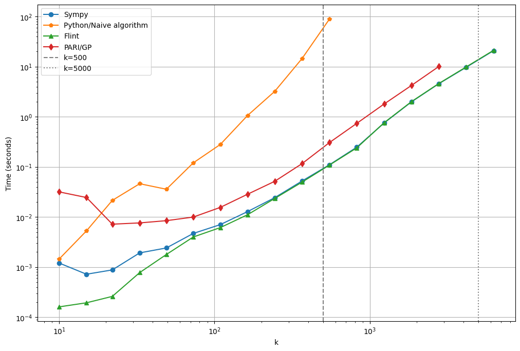
The general shape of the above plot confirms the \(O(n^2)\) time complexity of naive polynomial multiplication algorithm and the \(O(n \log n)\) time complexity of FFT-based multiplication algorithms used by modern libraries.
However, we also have an example of the more general phenomenon that a single time complexity is often not enough to yield important information - for example, comparing Sympy’s implementation of polynomial multiplication and flint’s implementation of polynomial multiplication, we can see different algorithms are used depending on the polynomial degree. These design choices ultimately explain the fact that Sympy is slower than Flint for small \(k\) but comparable for larger \(k\).
We showcase two techniques for calculating \(F(k)\) for higher \(k\).
Reconstruction via Chinese Remainder Theorem
Calculating the above polynomial in \(\mathbb{Z}[x]\) is slow mainly due to the size of the polynomial’s coefficients. Note that since all of the coefficients of \(x\) in \(p(x)\) are positive, we have that
\[F(k) \le \text{sum of all coefficients} = p(1) = 2^{4k} \cdot 3^{2k} \cdot 5^k = 720^k\]
We can remedy this by instead calculating the polynomial in \(\mathbb{Z}_p[x]\) for a small prime \(p\):

We then can calculate \(F(k) \bmod p\) for several small primes in parallel and then use the above bound with the Chinese Remainder Theorem to reconstruct the actual value of \(F(k)\).

We illustrate this by calculating \(F(50000)\). Since we know that \(F(50000) \le 720^{50000}\), we calculate \(F(50000) \bmod p\) for \(\frac{\log_{2}(720^{50000})}{64} \approx 7416\) 64-bit primes in parallel and then reconstruct the value of \(F(50000)\) with the Chinese Remainder Theorem:
from concurrent.futures import ProcessPoolExecutor
from math import log2
from sympy import nextprime, poly, GF
from sympy.abc import x
from sympy.ntheory.modular import crt
from tqdm import tqdm

import sys; sys.set_int_max_str_digits(10**6)

k = 50000
NUM_PRIMES = 1 + int( log2(720 ** k ) / 64 )

# Calculate first `NUM_PRIMES` 64-bit primes to use in CRT calculation
print(f"[+] Calculating {NUM_PRIMES} 64-bit primes")
primes = [nextprime(2**64)]
while len(primes) < NUM_PRIMES:
        primes.append(nextprime(primes[-1]))

# Note: We get massive speedup with python-flint being installed
# Otherwise, this is rather slow
def calc_f(k, MOD):
    p1 = x+1
    p2 = x**2+x+1
    p3 = x**4+x**3+x**2+x+1
    p = poly(p1, domain=GF(MOD))**(4*k) * poly(p2, domain=GF(MOD))**(2*k) * poly(p3, domain=GF(MOD))**k
    return ( p.coeff_monomial(x**(6*k)) % MOD, MOD)

# Worker function to pass to ProcessPoolExecutor
# Because lambdas can't be pickled?
def worker(p):
        return calc_f(k, p)

# Calculate F(k) mod p in parallel
print(f"[+] Calculating F({k}) mod primes")
results = []
with ProcessPoolExecutor(max_workers=32) as executor:
        futures = executor.map( worker, primes )
        for future in tqdm(futures, total=len(primes)):
                results.append(future)

# Reconstruct with CRT
print(f"[+] Reconstructing F({k})...")
res = str( crt([i[1] for i in results], [i[0] for i in results], check=False)[0] )
print(f"F({k}) = {res[:10]}...{res[-10:]} ({len(res)} digits)")
$ time python3 solve_crt.py
[+] Calculating 7416 64-bit primes
[+] Calculating F(50000) mod primes
100%|███| 7416/7416 [09:31<00:00, 12.97it/s]
[+] Reconstructing F(50000)...
F(50000) = 3612727222...0386752768 (142864 digits)
real 10m7.741s
user 303m3.718s
sys 2m2.420sFor more on algorithms of this kind, see Modern Computer Algebra by von zur Gathen and Gerhard Chapter 5.
Guessing A Closed Form
Instead of calculating all of the coefficients of \(p(x)\) for large \(k\) - we instead calculate only the coefficient of \(x^{6k}\). We use the standard notation for the coefficient of operator: \[ f(x) = \sum_{k \ge 0} a_k x^k \iff [x^k]f(x) = a_k \] We have: \[\begin{aligned} F(k) &= [x^{6k}] \left( (x+1)^{4k} (x^2+x+1)^{2k} (x^4+x^3+x^2+x+1)^k \right) \\ &= [x^{6k}] \left( \left( \frac{1-x^2}{1-x} \right)^{4k} \left( \frac{1-x^3}{1-x} \right)^{2k} \left( \frac{1-x^5}{1-x} \right)^{k} \right) \end{aligned}\]
Using the identities \((1-x^k)^\alpha = \sum_{i} \binom\alpha i (-1)^i x^{ik}\) and \((1-x)^{-k} = \sum_i \binom{i+k-1}{i} x^i\), we have:
\[\begin{aligned} F(k) &= [x^{6k}] \left( (1-x^2)^{4k} \cdot (1-x^3)^{2k} \cdot (1-x^5)^k \cdot (1-x)^{-7k} \right) \\ &= [x^{6k}] \left( \left( \sum_a \binom{4k}{a} (-1)^a x^{2a} \right) \left( \sum_b \binom{2k}{b} (-1)^b x^{3b} \right) \left( \sum_{c} \binom{k}{c} (-1)^c x^{5c} \right) \left( \sum_d \binom{d+7k-1}{d} x^d\right) \right) \\ &= \sum_{2a+3b+5c+d = 6k} \binom{4k}{a} \binom{2k}{b} \binom{k}{c} \binom{d+7k-1}{d} (-1)^{a+b+c} \\ &= \sum_{a,b,c} \binom{4k}{a} \binom{2k}{b} \binom{k}{c} \binom{13k-5c-3b-2a-1}{6k-5c-3b-2a} (-1)^{a+b+c} \end{aligned}\]
This representation as a summation suggests that \(F(k)\) may have a closed form or at least a simple recurrence. We attempt to guess such a closed form with SageMath (see this paper for the package used):
sage: R.<x> = PolynomialRing(QQ)
sage: def F(k):
....:     p = (x+1)**(4*k) * (x**2+x+1)**(2*k) * (x**4+x**3+x**2+x+1)**k
....:     return p.coefficients()[6*k]
sage: seq = [F(k) for k in range(200)]
sage: C = CFiniteSequences(QQ); C.guess(seq)
0 # Sequence is likely not defined by a linear recurrence
sage: from ore_algebra import OreAlgebra, guess
sage: g = guess(seq, OreAlgebra(QQ['n'], 'Sn'))
sage: [ p.degree() for p in g ]
[18, 18, 18, 18, 18]
sage: %time seq_more = g.to_list(init=seq[:5], n = 100000) # Calculate the first 100000 terms
# CPU times: user 2min 21s, sys: 1.06 s, total: 2min 22s
# Wall time: 2min 22s
sage: test = str(seq_more[50000]) # Compare to F(50000) value calculated before
sage: f"F(50000) = {test[:10]}...{test[-10:]} ({len(test)} digits)"
'F(50000) = 3612727222...0386752768 (142864 digits)'
Problem 5
What is the largest zero of the 1000th Laguerre polynomial to 12 significant digits? - the Laguerre polynomials satisfy the recurrence relation \[\begin{cases} L_0(x) = 1 \\ L_1(x) = 1-x \\ L_n(x) = \frac{2n-1-x}{n}L_{n-1}(x) - \frac{n-1}{n} L_{n-2}(x) & n > 1 \end{cases}\]
Naive Approach
Direct calculation with numpy yields numerical
overflow:
import numpy as np
from scipy.special import laguerre

L = laguerre(1000)
all(np.isnan(L))
# /usr/local/lib/python3.12/dist-packages/scipy/special/_orthogonal.py:568: RuntimeWarning: overflow encountered in multiply
#  - (n + alpha) * _ufuncs.eval_genlaguerre(n - 1, alpha, x)) / x

# True
Explicitly, the \(n^\text{th}\) Laguerre polynomial can be written as \(L_n(x) = \sum_{k=0}^n \binom{n}{k} \frac{(-1)^k}{k!}x^k\) - therefore, the higher order coefficients will be too small to be representable in floating point.
Root Isolation
Given a polynomial, Sage has built-in functionality to calculate a list of intervals containing all of its real roots - we demonstrate this functionality below:
sage: R.<x> = QQ[]
....: n = 1000
....: P = sum([binomial(n, k)*(-1)^k/factorial(k)*x^k for k in range(n
....: +1)])
....: P *= P.denominator()
....: # Calculate interval where maximum root lies
....: (lo, hi), _ = P.real_root_intervals()[-1]
....: # Do binary search to refine interval
....: while abs(hi - lo) > 10**(-12):
....:     print(".", end="")
....:     mid = (lo + hi)/2
....:     if P(mid) * P(lo) > 0:
....:         lo = mid
....:     else:
....:         hi = mid
....: print("\n", mid.n() )
.............................................
3943.24739484527
Problem 6
Find both the global maximum of \(J_\nu(2000 \pi)\) and where it occurs. Compute the global maximum to 16 significant digits, and compute where it occurs to 8 significant digits.
- here, we restrict \(\nu \ge 0\)
- \(J_\nu\) is the Bessel function of the first kind
Some Theory
Before solving the problem, we should take a second to determine whether or not the problem is well-posed, as it is not clear whether or not this function even has a maximum in the first place.
However, note that we have that for fixed \(z\) and as \(\nu \to \infty\), we have \[J_{\nu}\left(z\right)\sim\frac{1}{\sqrt{2\pi\nu}}\left(\frac{ez}{2\nu}\right)^{\nu} \to 0\]
We also have the strict inequality
\[ | J_\nu(x)| \le \frac{1}{\Gamma(\nu+1)} \left(\frac{x}{2}\right)^\nu \implies |J_\nu(2000\pi)| \le \underbrace{ \frac{(1000\pi)^\nu}{\Gamma(\nu+1)} }_{f(\nu)}\]
It can be shown that for large enough \(N\) - say \(10^4\) - \(f(\nu)\) is decreasing on \((N, \infty)\). We therefore have that for \(\nu > 10^4\) that
\[|J_\nu(2000 \pi)| \le f(10^4) \approx 1.11 \cdot 10^{-688}\]
It therefore suffices to find the optimum \(\nu^* = \arg\max_{\nu \in [0, 10000] } J_\nu(2000\pi)\). We find this optimum with brute force:
from scipy.optimize import minimize, brute, fmin
from scipy.special import jv
from math import pi

F = lambda v: -jv(v, 2000*pi)

res = brute(
     lambda v: -jv(v, 2000*pi),
    (slice(0, 10000, 0.01), ), full_output=True, disp=True, finish=fmin)

# (array([6268.26082196]), -0.03658537275397168)
Problem 7
Define functions \(f(x)\) and \(g(x)\) as
\[\begin{aligned} f(x) &= \tan(\tanh(\sin(x))) + \tanh(\sin(\tan(x))) \\ &+ \sin(\tan(\tanh(x))) - \tan(\sin(\tanh(x))) \\ &- \sin(\tanh(\tan(x))) - \tanh(\tan(\sin(x))) \\ &- \tan(\sinh(\tanh(x))) - \sinh(\tanh(\tan(x))) \\ &- \tanh(\tan(\sinh(x))) + \tan(\tanh(\sinh(x))) \\ &+ \tanh(\sinh(\tan(x))) + \sinh(\tan(\tanh(x))) \end{aligned}\]
and
\[\begin{aligned} g(x) &= \sinh(\tanh(\sin(x))) + \tanh(\sin(\sinh(x))) \\ &+ \sin(\sinh(\tanh(x))) - \sinh(\sin(\tanh(x))) \\ &- \sin(\tanh(\sinh(x))) - \tanh(\sinh(\sin(x))) \\ &- \tan(\sinh(\sin(x))) - \sinh(\sin(\tan(x))) \\ &- \sin(\tan(\sinh(x))) + \tan(\sin(\sinh(x))) \\ &+ \sin(\sinh(\tan(x))) + \sinh(\tan(\sin(x))) \end{aligned}\]
What is \(\lim_{x \to 0} \frac{f(g(x))}{g(f(x))}\) to 9 significant digits?
Naive Approach
Direct evaluation of \(f(x)\) is
suceptible to underflow - this problem compounds when calculating \(f(g(x))\) and \(g(f(x))\). Hence, directly calculating
\(\frac{f(g(x))}{g(f(x))}\) is not
feasible except for \(x \approx 0.9\)
even with extended 128-bit precision. 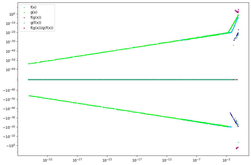
Power Series
Instead of directly evaluating \(f\) and \(g\), note that at \(z=0\), we have the series expansions:
\[ \begin{aligned} \sin z &= \sum_{k=0}^{\infty} \frac{(-1)^k z^{2k+1}}{(2k+1)!} \\ \sinh{z} &=\sum_{k=0}^{\infty} \frac{z^{2k+1}}{(2k+1)!} \\ \tan{z} &= \sum_{k=1}^{\infty} \frac{(-1)^{k-1}(2^{2k} - 1)2^{2k} B_{2k} z^{2k-1}}{(2k)!} \\ \tanh{z} &= \sum_{k=1}^{\infty} \frac{(2^{2k} - 1)2^{2k} B_{2k} z^{2k-1}}{(2k)!} \end{aligned} \]
We can therefore calculate \(F(x) = f(g(x)) / g(f(x))\) as a formal power series - this can be done in a couple lines of SageMath
sage: R.<x> = PowerSeriesRing(QQ, default_prec = 20)
....: f = tan(tanh(sin(x))) + tanh(sin(tan(x))) + sin(tan(tanh(x))) - tan(sin(tanh(x))) - sin(tanh(tan(x))) - tanh(tan(sin(x))) - tan(sinh(tanh(x))) - sinh(tanh(tan(x))) - tanh(tan(sinh(x))) + tan(tanh(sinh(x))) + tanh(sinh(tan(x))) + sinh(tan(tanh(x)))
....: g = sinh(tanh(sin(x))) + tanh(sin(sinh(x))) + sin(sinh(tanh(x))) - sinh(sin(tanh(x))) - sin(tanh(sinh(x))) - tanh(sinh(sin(x))) - tan(sinh(sin(x))) - sinh(sin(tan(x))) - sin(tan(sinh(x))) + tan(sin(sinh(x))) + sin(sinh(tan(x))) + sinh(tan(sin(x)))
sage: f(g(x)) / g(f(x))
2451447860952057740817096729600000000000000000000/801034487517232030831498951509084442801 + 268594208861616474527619350824913280000000000000000000/6223236933521375647529915354274077036120969*x^4 + O(x^5)
As we have that \(F(x) = c_0 + c_1 x^4 + \cdots\), we have that \(\lim_{x \to 0} F(x)\) is the constant term in the above power series, namely
\[ \frac{2451447860952057740817096729600000000000000000000}{801034487517232030831498951509084442801} \approx 3060352455.6729174 \]
Problem 8
What is
\[\prod_{n=1}^\infty \tanh\left( \frac{1}{2} \tan^{-1}(n) \sinh^{-1}(n)\right)\]
to 14 significant digits?
Initial Attempts

Note that the terms of the product rapidly approach 1 - hence, we can get an estimate of the above product by taking a partial product.
We can write a simple C program to take the product of the first N terms:
#include<stdio.h>
#include<math.h>

double F(int n) {
    return tanh(0.5 * atan(n) * asinh(n));
}

int main(int argc, char** argv) {
    double out = 1;
    int lim = atoi( argv[1] );
    for (int i = 1; i < lim; i++) {
        out *= F(i);
    }
    printf("%d: %.17lf\n", lim, out);
}
$ for i in {0..32..2}; do ./calc_prod "$((1 << i)) "; done; echo
1: 1.00000000000000000
4: 0.17959494132937540
16: 0.11082394271675355
64: 0.09462337598787798
256: 0.08879820894851700
1024: 0.08637294794296040
4096: 0.08530853193572750
16384: 0.08483213403121476
65536: 0.08461730643287897
262144: 0.08452014245788493
1048576: 0.08447614250058469
4194304: 0.08445620714072524
16777216: 0.08444717286874558
67108864: 0.08444307833008752
268435456: 0.08444122251122592
1073741824: 0.08444038143574970With this, we get that the product is approximately \(0.08444\)
More Digits
First, note we have: \[ \begin{aligned} L = \prod_{n=1}^\infty F(n) &\implies \ln(L) = \sum_{n=1}^\infty \ln(F(n)) \\ &= \underbrace{ \sum_{k=1}^N \ln(F(n)) }_{\text{calculate}} + \underbrace{ \sum_{k > N} \ln(F(n)) }_{\text{estimate }} \end{aligned} \]
To get more digits, we utilize the Abel-Plana formula - this is similar to the Euler-Macluarin summation formula mentioned earlier; however, as mentioned in mpmath’s documentation, Abel-Plana works better when the growth of \(F(k)\) above grows like a power of \(k\) as we have here.
import mpmath
from mpmath import log, tanh, atan, asinh, inf

mpmath.mp.dps = 100
F = lambda n: log( tanh( 0.5 * atan(n) * asinh(n) ) )
N = 500

sum1 = sum( [F(i) for i in range(1, N)] ) # Sum first N terms
sum2, err = mpmath.sumap( F, [N, inf], error=True) # Get bound on tail

# Calculate total product via interval arithmetic
mpmath.iv.dps = 100
# sum of F(k) for k > 0 is bounded by below interval
sum_interval = mpmath.iv.mpf( [ sum1 + sum2 - err, sum1 + sum2 + err ])
prod_interval = mpmath.iv.exp( sum_interval )
mpmath.mpf( prod_interval.a ), mpmath.mpf( prod_interval.b )

# 0.0844396840301890445961951627743214644576628...
# 0.0844396840301890445961951627743214644576796...
With the above method, we are able to get 42 correct significant digits.
Problem 9
Find the largest eigenvalue \(\lambda\) to 13 significant digits for the following integral equation. \[ \int_0^1 \exp(x + y + x^2 + xy + y^2 + x^2 y^2 ) f(y) dy = \lambda f(x) \]
Initial Setup
Note that this is an example of a Fredholm integral equation of the second kind. For ease of notation, let $K(x,y) = (x + y + x^2 + xy + y^2 + x^2 y^2 ) $ be the kernel that \(f\) is integrated against, and let \(g(x,y) = K(x,y) f(y)\) be the integrand in the left hand side above.
We can use any number of quadrature rules to approximate the integral on the right hand side - for sample points \(0 \le y_1 < y_2 \cdots < y_{N-1} < y_N \le 1\) and weights \(\{ w_j \}_{1 \le j \le N}\), we have \[ \int_0^1 g(x,y) dy \approx \sum_{j=1}^N w_j g(x, y_j) \]
The above equation therefore becomes \[ \lambda f(x) \approx \sum_{j=1}^N w_j K(x, y_j) f(y_j) \\]
Assume we sample \(f\) at \(N\) points \(0 \le x_1 < x_2 \cdots x_{N-1} < x_N \le 1\). For each \(x_i\) and taking each above approximation above as an equality, we get \(N\) equations. \[ \lambda f(x_i) = \sum_{j=1}^N w_j K(x_i, y_j) f(y_j) \]
We rewrite the above system using matrices: let - $ K = [K(x_i, y_j)]{1 i,j N} ^{NN}$ be a matrix of the kernel at the chosen sample points - $ w = [w_j]{1 j N}$ be a vector of weights given by the chosen quadrature rule - \(f = [f(x_k)]_{1 \le k \le N}\) be the vector of function values which we aim to solve for
After expanding, the above equation becomes: \[\begin{aligned} \underbrace{ \begin{bmatrix} \lambda f(x_1) \\ \vdots \\ \lambda f(x_n) \end{bmatrix}}_{\lambda f} &= \begin{bmatrix} \sum_{j=1}^N w_j K(x_1, y_j) f(y_j) \\ \vdots \\ \sum_{j=1}^N w_j K(x_1, y_j) f(y_j) \end{bmatrix} \\ &= \sum_{j=1}^N \left( (f(y_j ) \cdot \begin{bmatrix} K(x_1, y_j) w_j \\ \vdots \\ K(x_n, y_j) w_j \end{bmatrix} \right) \\ &= \underbrace{ \begin{bmatrix} K(x_1, y_1) w_1 & \cdots & K(x_1, y_n) w_1 \\ \vdots & \ddots & \vdots \\ K(x_n, y_1) w_n & \cdots & K(x_n, y_n) w_n\end{bmatrix} }_{\hat{K}} \begin{bmatrix} f(y_1) \\ \vdots \\ f(y_n) \end{bmatrix} \\ &= \hat{ K }f \\ \implies \lambda f = \hat{K} f \end{aligned}\]
Small technicality: In the above and what follows, we assume that \(x_i = y_i\) for all \(1 \le i \le N\).
Note that finding the eigenvalues of the matrix \(\hat{K} \in \R^{N \times N}\) takes \(O(N^3)\) time complexity - we therefore want a quadrature rule with minimal sample points. To illustrate this, we use the above method with two different quadrature rules: - we use Simpson’s 3/8 rule - we have:
\[\begin{aligned} \int_0^1 f (x) dx \approx \frac{3}{8N} &( f(x_0) + 3f(x_1) + 3f(x_2) \\ + 2&f(x_3) + 3f(x_4) + 3f(x_5) \\ &+ \cdots + \\ + 2&f(x_{n-3}) + 3f(x_{n-2}) + 3f(x_{n-1}) \\ +&f(x_n)) \end{aligned} \]